How do I assign words to values in excel?

[purplepoppy]

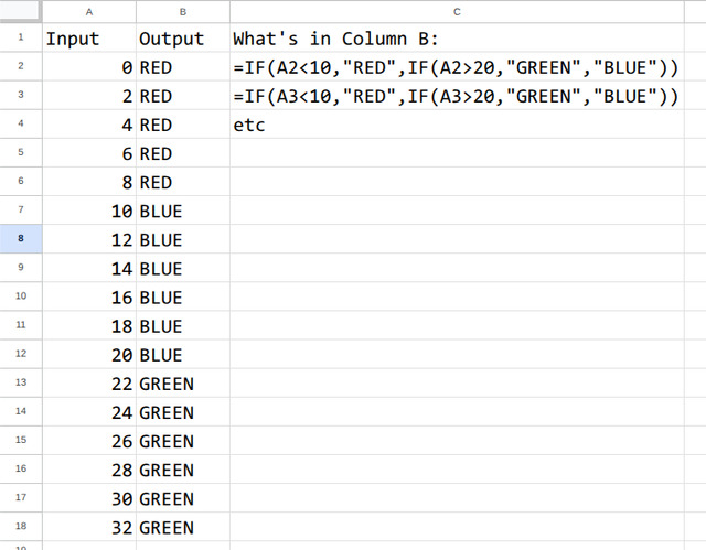
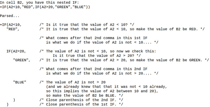
I'm looking to use excel to assign various words according to where values fall between ranges.
Eg if <10 red
If between 10 and 20 blue
If >20 greens

I've been messing with the IF command but its not coming out as I want

[SueShe]

Have you tried the IFS instead of IF or VLOOKUP or XLOOKUP or even the SWITCH functions in E***l. You may find a few explanation and tutorial videos on a popular video site that could help you with your problem.

You can probably also find a tutorial in one popular Q&A site. If all fails, you can try to contact the manufacturer of that software if you are a registered user of that specific software program.

Good luck as this is the only help I can try to provide. I am not a specialist and I never came across that type of formula.

[OneViewpoint]

Conditional formatting. You don't write a formula in the cell like =A1 + B1.

You go into "Home" on the ribbon at the top of the screen. Then the styles section of the home ribbon. You'll see "Conditional Formatting" as the first option. Click on that.

You'll see a list of options for creating rules for formatting the cell based on its result. Some common things are premade for you like > and <. Or you can you to "New Rule" near the bottom of the list and write more complex logic. You can use fill colors, data bars, or icons as out of the box cell highlights. Or you can write your own code to display anything you want. Easy peasy.

[OneViewpoint]

If you write your own rules, you can insert any text you want as the conditional formatting. For instance "Cool" and "Not Cool".

[goaded]

=IFS (D14>20,"Red", D14>10,"Amber",1,"Green")

Shows Red for D14>20, Amber 11-20, otherwise (1 = true), Green.

That's LibreOffice, but it might work in Excel.

[purplepoppy]

Thanks

[goaded]

Thank @SueShe, I just looked up IFS! I haven't much of a clue about spreadsheets, although I'm in awe of the genius who invented them, and allowed anyone to freely use his work.

[exitseven]

Try this
SWITCH Function (Cleanest Formula)
Similar to IFS, SWITCH is efficient for mapping specific text to specific values.
Formula: =SWITCH (A2,"Low",10,"Medium",20,"High",30)
This function evaluates A2 and returns the value assigned to the matching te

[Jersey2]

You could try and feed it into Grok in a file and it to recommend a fix or fix it. Better yet, you could use an AI to create a new program outside of Excel to process the information. I would start by asking Grok which AI are best suited for this and then watch some Youtube videos on it and then given it a go.

[Jersey2]

And ask it*

[jshm2]

If you want to go down the IFS route then try =IFS (A2<10,"red", A2<=20,"blue", A2>20,"green")

else =IF (A2<10,"red", IF (A2<20,"blue","green"))

[MrChinaski]

ChatGPT will give you all the code you need to enter.

If statements would suffice. I'm sure it can do better.

[Shiprex]

=if (#NUM<10, "RED", if (#NUM>20,"GREENS","BLUE"))

[Anonymous]

You should probably check out some Excel manual.

[abc3643]

Conditional Formatting
Home tab

[abc3643]

I may be misunderstanding you though. Can you be more explicit?

[abc3643]

MY FUCKING CAT DESTROYED MY ANSWER!

OK, look, I've run out of time to retype my magnum opus...

This is the answer and it will involve nesting IF functions.

Assume A2 is the cell whose value you are going to check.
Assume B2 is the cell whose value is going to take on RED, GREEN, or BLUE, based on the value of cell A2.

=IF (A2<10,"RED", IF (A2>20,"GREEN","BLUE"))

Proof it works:


Now, try to figure out WHY it works...

Maybe I can help by parsing the answer...



If you have any questions, feel free to ask.

Now, I gotta tell you, we got away with this nested IF because we had only 3 "cases": <10 is red, >20 is green, and between them is blue. If we have several cases, then it becomes rather cumbersome to use nested IFs and one can even run into a limit of how many nested IFs you can have. In that case, we'd have to do something else.

[purplepoppy]

Thanks

[Nikki1989]

Use a lookup table.

[Jennz6]

That’s way too much for me